Chapter 7 — Laplace's Equation

Quote

“The problem of finding the solution to any electrostatic problem is equivalent to finding a solution of Laplace’s equation throughout the space not occupied by conductors.”

— Sir James Jeans (1925)

Motivation

The Coulomb integral

$$\phi (\mathbf{r})=\frac{1}{4\pi {ϵ}_0}\int {\mathrm{d}}^3{r}^{\prime }\frac{\rho (\mathbf{r}{}^{\prime })}{|\mathbf{r}-\mathbf{r}{}^{\prime }|}$$

loses its utility when $\rho (\mathbf{r})$ cannot be specified once and for all. However, we do know how conductors and simple dielectrics behave in electrostatic fields. Potential theory covers exactly this situation: the Poisson equation ${\nabla }^2\phi =-\rho /{ϵ}_0$, continuity of $\phi$, discontinuity of $\partial \phi /\partial n$ across an interface (with outward normal ${\hat{\mathbf{n}}}_2$ pointing from region 1 into region 2):

$${\kappa }_1\frac{\partial {\phi }_1}{\partial n_2}-{\kappa }_2\frac{\partial {\phi }_2}{\partial n_2}=\frac{{\sigma }_f}{{ϵ}_0}$$

and boundary conditions.

Getting comfortable with this machinery pays off: it yields interesting analytical solutions, and these also serve as limiting cases and checks for numerical work.

---

Uniqueness

Key Physical Idea

A solution to Poisson’s equation is unique in vacuum or simple-dielectric regions bounded by conductors. This permits a “guessing” strategy: if you find any solution satisfying the PDE and BCs, it is the solution.

We limit ourselves to situations where surface charge densities account for all the charge in the system — i.e., we solve Laplace’s equation at points that do not lie on the charged surfaces.

If those surface charges are known, then either integrating Coulomb’s formula or knitting together solutions of Laplace’s equation will give the solution that is unique by the Helmholtz theorem. Usually, $\sigma ({\mathbf{r}}_S)$ is not known and we use potential theory to find $\phi (\mathbf{r})$ first, then calculate the $\sigma$s using matching conditions (which would reproduce $\phi$ by uniqueness).

Uniqueness Proof Sketch

Setup: Connected volume $V$ bounded by any number of non-overlapping closed surfaces $S_1,S_2,\dots$ and an outer enclosing surface $S_{\infty }$.

Assume two solutions ${\phi }_1,{\phi }_2$ satisfying the same BCs, and let $\Phi ={\phi }_1-{\phi }_2$. Apply Green’s first identity ${\int }_V{\mathrm{d}}^{3}r\left(f{\nabla }^{2}g+\nabla f\cdot \nabla g\right)={\int }_S\mathrm{d}\mathbf{S}\cdot f\nabla g$ with $f=g=\Phi$:

$${\int }_V{\mathrm{d}}^{3}r|\nabla \Phi {|}^2=\sum _i{\oint }_{S_i}d\mathbf{S}\cdot \Phi \nabla \Phi$$

The left side is manifestly non-negative. Choose BCs that force the right side to vanish:

Condition	Specification	Why RHS vanishes
Dirichlet	$\phi ({\mathbf{r}}_S)$ given	$\Phi =0$ on all surfaces
Neumann	$\hat{n}\cdot \nabla \phi ({\mathbf{r}}_S)$ given	$\hat{n}\cdot \nabla \Phi =0$ on all surfaces
Mixed	Dirichlet on some surfaces, Neumann on others	Each surface contributes zero independently

In all cases ${\int }_V{\mathrm{d}}^{3}r|\nabla \Phi {|}^2=0⟹\nabla \Phi =0$ throughout $V$, so ${\phi }_1={\phi }_2$ (up to an irrelevant constant for Neumann).

Only one type of condition (Dirichlet or Neumann) should be specified at each surface point. Specifying both is either redundant or inconsistent.

For unbounded problems, the enclosing surface $S_{\infty }$ recedes to infinity. A fall-off condition like $\phi \to 0$ as $r\to \infty$ serves as the Dirichlet condition on this surface.

Conductors: Charge Specification

Conductor Uniqueness (Jeans' Extension)

If the surfaces are conducting, the solution is unique if for every conductor we specify either its potential (Dirichlet) or its total charge — even though total charge is less information than a full Neumann condition.

Proof: Why Total Charge Suffices

On a conductor $S_k$, $\phi$ is constant, so

$${\oint }_{S_k}d\mathbf{S}\cdot \Phi \nabla \Phi =({\phi }_1-{\phi }_2){\oint }_{S_k}d\mathbf{S}\cdot (\nabla {\phi }_1-\nabla {\phi }_2)=-\frac{1}{{ϵ}_0}({\phi }_1-{\phi }_2)(Q_1-Q_2)$$

where $Q_{1,2}=-{ϵ}_0{\oint }_{S_k}\frac{\partial {\phi }_{1,2}}{\partial n}dS$. If we specify $Q$, then $Q_1=Q_2$ and this vanishes.

Physical Consequence

This explains why the electric field outside a perfect conductor is independent of how charge is distributed inside a cavity — only the total charge matters. The amount $Q$ induced on the inner cavity surface shields the interior, so only $Q_{\text{total}}$ affects the exterior.

Example: A point dipole inside a conducting cavity produces zero field outside (total conductor charge is zero).

These two specifications (potential vs. total charge) are exclusive alternatives: from knowing $\phi$ everywhere we can integrate for the $Q_k$, or use the capacitance matrix for the other direction.

Why the Special Conductor Argument?

One might ask: doesn’t the general uniqueness theorem already cover everything? The point is that conductors represent a special physical case: we often know total charge in practice rather than the full surface potential or normal derivative. The conductor extension proves that this hybrid condition ($Q$ + the fact that conductors are equipotentials) suffices for uniqueness in that important case.

Scope of Different BC Types

Dirichlet BCs cover the most common situations: only dielectric matter and/or conductors present.

Neumann BCs arise in more specialized settings:

• Steady current through an ohmic medium (link): no current ($\propto \mathbf{E}\sim \nabla \phi$) flows out of the medium, so $\hat{n}\cdot \nabla \phi =0$;
• Superconductors (link): Meissner effect requires that the magnetic potential gradient vanishes at the surface.

Mixed BCs require exotic methodology (cf. Morse & Feshbach). Example: a half-covered electrode.

---

Separation of Variables

Many problems have a symmetry that makes a particular coordinate system natural. In orthogonal coordinate systems, we split the solution:

$$\phi (u,v,w)=A(u)B(v)C(w)\text{.}$$

The 13 Separable Coordinate Systems

Laplace’s equation is separable in exactly 13 orthogonal coordinate systems: Cartesian, cylindrical, spherical, conical, bispherical, ellipsoidal, parabolic cylindrical, elliptic cylindrical, oblate spheroidal, prolate spheroidal, parabolic, paraboloidal, and toroidal.

Separation yields three second-order ODEs with dependent separation constants. The approach: determine the functions and coefficients, and the nature of the separation constants (integer, real, imaginary) from:

1. Symmetries of the problem
2. Boundary conditions
3. Finiteness throughout the solution volume

Discrete vs. Continuous Spectra

• Bounded direction with homogeneous BCs → discrete modes (eigenvalue problem on a finite interval)
• Unbounded direction → continuous spectrum (Fourier integrals)

Finiteness requirements are what discretize the separation constants.

Completeness

A set of functions $\{{\varphi }_k(v)\}$ on $a\le v\le b$ is complete if any function on the same interval can be expanded as their linear combination. This is conveniently stated as the closure relation:

$$\sum _k{\varphi }_k(v){\varphi }_k^{\ast }(v^{\prime })=\delta (v-v^{\prime })\text{,}$$

which implies completeness via $F(v)={\int }_a^b\mathrm{d}{v}^{\prime }\delta (v-v^{\prime })F(v^{\prime })$, and also gives the orthonormality relation:

$${\int }_a^b\mathrm{d}v{\varphi }_k^{\ast }(v){\varphi }_j(v)={\delta }_{kj}\text{.}$$

---

Cartesian Coordinates

Separation $\phi (x,y,z)=X(x)Y(y)Z(z)$ gives:

$$\frac{X^{\prime \prime }}{X}={\alpha }^2,\frac{Y^{\prime \prime }}{Y}={\beta }^2,\frac{Z^{\prime \prime }}{Z}={\gamma }^2,{\alpha }^2+{\beta }^2+{\gamma }^2=0\text{.}$$

Each factor is either:

• $A+Bx$ (if separation constant is zero), or;
• $A_{\alpha }{e}^{\alpha x}+B_{\alpha }{e}^{-\alpha x}$ (equivalently, $\sinh /\cosh$ or $\sin /\cos$).

The constraint ${\alpha }^2+{\beta }^2+{\gamma }^2=0$ means $\alpha ,\beta ,\gamma$ cannot all be purely real or all purely imaginary. In most cases, at least one is real and at least one is imaginary. It yields a (possibly continuous) family of solutions, which can be superposed by linearity.

Example: Grounded box with one hot wall

A box of dimensions $a\times b\times c$ has $z=0$ wall held at potential $V(x,y)$; all other walls are grounded.

Homogeneous BCs in $x$ and $y$ immediately select:

$$X_m(x)=\sin \left(\frac{m\pi x}{a}\right),Y_n(y)=\sin \left(\frac{n\pi y}{b}\right)$$

The $z$-dependence must vanish at $z=c$:

$$Z_{mn}(z)=\frac{\sinh ({\gamma }_{mn}(c-z))}{\sinh ({\gamma }_{mn}c)},{\gamma }_{mn}=\pi \sqrt{\frac{m^2}{a^2}+\frac{n^2}{b^2}}$$

Full solution:

$$\phi (x,y,z)=\sum _{m=1}^{\infty }\sum _{n=1}^{\infty }{V}_{mn}\sin \left(\frac{m\pi x}{a}\right)\sin \left(\frac{n\pi y}{b}\right)\frac{\sinh ({\gamma }_{mn}(c-z))}{\sinh ({\gamma }_{mn}c)}\text{,}$$

where the coefficients follow from orthogonality on the $z=0$ face:

$$V_{mn}=\frac{4}{ab}{\int }_0^a\mathrm{d}x{\int }_0^b\mathrm{d}yV(x,y)\sin \left(\frac{m\pi x}{a}\right)\sin \left(\frac{n\pi y}{b}\right)\text{.}$$

Faraday Cage (Parallel-Plate Wire Mesh)

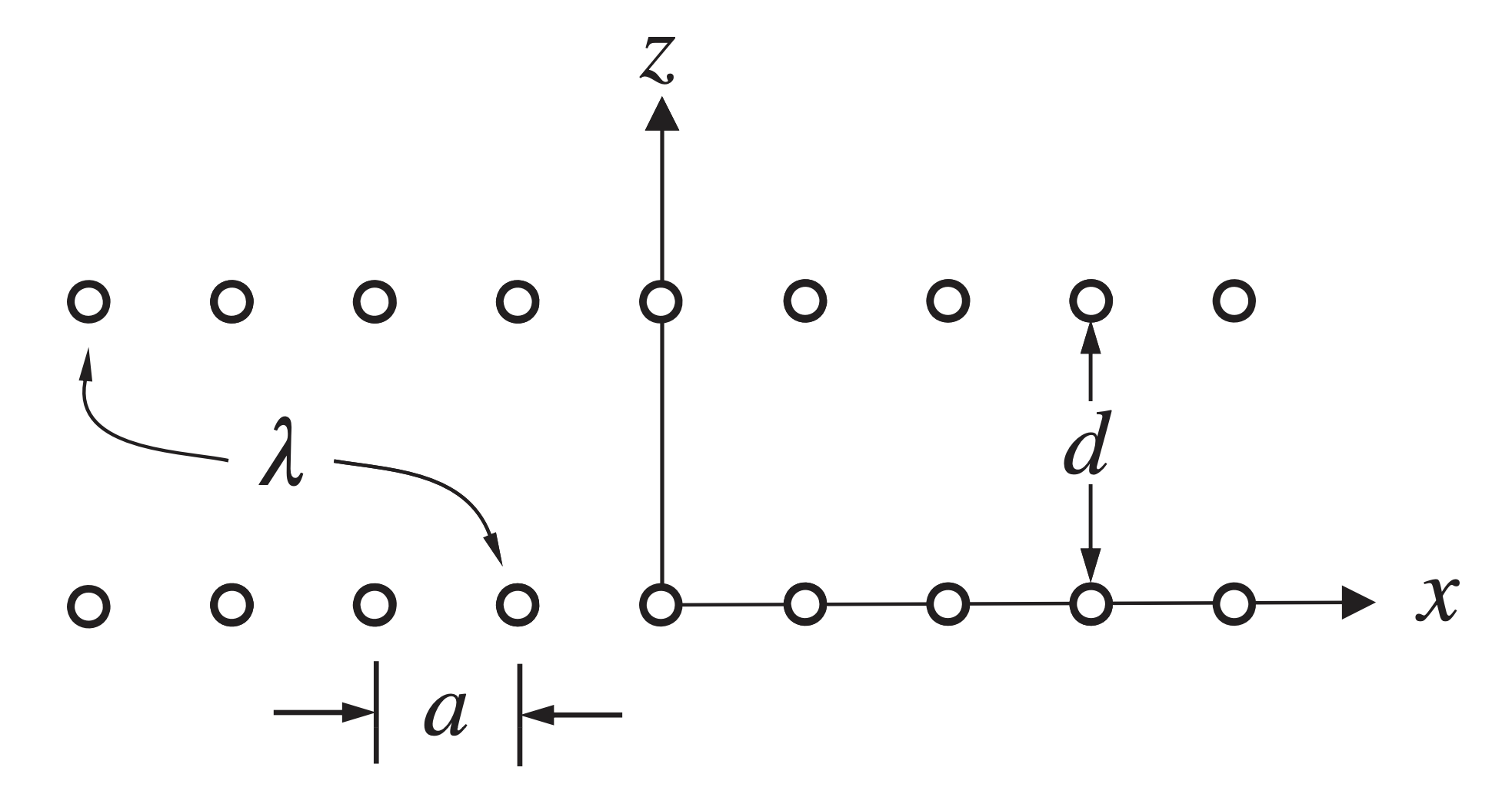
A cage made of parallel wires with spacing $a$ between two plates separated by $2d$.

Symmetries:

• $\phi (-x,-z)=\phi (x,z)$;
• Periodicity: $\phi (x+a,z)=\phi (x,z)$ → discretizes the separation constant.

Far from mesh ($|z|\gg a$): ordinary parallel-plate capacitor, $\phi \to A+B|z|$.

Near mesh: separation (no $y$-dependence) gives corrections of the form ${\sum }_{\gamma }{C}_{\gamma }\cos (\gamma x)e^{-\gamma |z|}$.

The $|z|$ from Separation

Laplace’s equation holds in three regions (above mesh, below mesh and inside it). In each region the $z$-solutions are ordinary exponentials. Writing the combined result as $e^{-\gamma |z|}$ is just the compact way to express the solution that decays away from the mesh in both directions. The matching condition at $z=0$ is:

$${\frac{\partial \phi }{\partial z}|}_{0^{-}}-{\frac{\partial \phi }{\partial z}|}_{0^{+}}=\frac{\sigma (x)}{{ϵ}_0},\sigma (x)=\lambda \sum _p\delta (x-pa)$$

Periodicity forces ${\gamma }_m=2\pi m/a$, and the result is that outside the mesh corrections decay as $e^{-2\pi m|z|/a}$:

$${\phi }_{\text{correction}}\sim \frac{\lambda }{2\pi {ϵ}_0}\sum _{m=1}^{\infty }\frac{1}{m}\cos \left(\frac{2\pi mx}{a}\right)e^{-2\pi m|z|/a}$$

Why $d\gg a$ is Required

All practical Faraday cages need $d\gg a$. Mathematically: the correction terms decay on scale $a/(2\pi )$. For the interior to truly look like a parallel-plate capacitor (just the linear $|z|$ term), the mesh-to-plate distance $d$ must be large enough that these corrections are negligible at the plates. If $d\sim a$, the “cage” is really just an array of wires and shielding is poor.

Earnshaw’s Theorem and Curvature

Geometric Interpretation of Laplace's Equation

${\nabla }^2\phi =0$ means the total curvature of $\phi (\mathbf{r})$ vanishes: ${\partial }^2\phi /\partial x^2+{\partial }^2\phi /\partial y^2+{\partial }^2\phi /\partial z^2=0$. All three 1D curvatures cannot have the same algebraic sign. This gives a qualitative understanding of Earnshaw’s theorem: a potential maximum or minimum (where all curvatures would be negative/positive) is impossible.

Corollary: Laplace solutions are unbounded in at least one Cartesian direction — but in examples like the Faraday cage, divergences signal regions where charge resides and Laplace’s equation ceases to hold.

---

Spherical Coordinates

Azimuthal Symmetry

With no $\varphi$-dependence, the reduced Laplacian gives two ODEs. The radial part:

$$R_{\nu }(r)=A_{\nu }{r}^{\nu }+B_{\nu }{r}^{-(\nu +1)}\text{.}$$

The angular part ($x=\cos \theta$):

$$\frac{\mathrm{d}}{\mathrm{d}x}\left[(1-x^2)\frac{\mathrm{d}M}{\mathrm{d}x}\right]+\kappa M=0,\kappa =\nu (\nu +1)\text{.}$$

Two linearly independent solutions: Legendre polynomials of first ($P_{\nu }(x)$) and second ($Q_{\nu }(x)$) kind.

$P_{\nu }$ (Legendre of 1st kind)	$Q_{\nu }$ (Legendre of 2nd kind)
$P_0=1,P_1=x,P_2=\frac{1}{2}(3x^2-1)$	$Q_0=\frac{1}{2}\ln \frac{1+x}{1-x},Q_1=x{Q}_0-1$
Finite on $[-1,1]$	Logarithmic singularities at $x=\pm 1$
Regular at both poles	Only for problems excluding the $z$-axis (e.g., between two coaxial cones with common vertex that open up in the same direction)

Non-Integer $\nu$

For $\nu \notin \mathbb{Z}$, $P_{\nu }(x)={}_2{F}_1(-\nu ,\nu +1;1;(1-x)/2)$ has a branch-point singularity at $x=-1$. The hypergeometric series terminates (becoming a polynomial) only when $\nu$ is a non-negative integer — precisely the Legendre polynomials, finite on all of $[-1,1]$.

Non-integer $\nu$ arises for conical boundaries, wedge domains, exterior of a cone, etc.

Generating Function Trick: On-Axis → Full Solution

The generating function for Legendre polynomials:

$$\frac{1}{\sqrt{1-2xt+t^2}}=\sum _{\ell =0}^{\infty }{t}^{\ell }{P}_{\ell }(x),|x|\le 1,0<t<1$$

On the symmetry axis, $P_{\ell }(1)=1$, so any azimuthally symmetric potential is uniquely determined by its values on the symmetry axis. Find $\phi (0,0,z)$ by elementary means, expand in powers of $z$ (or $1/z$), and read off the coefficients.

Example — Charged Ring

Total charge $Q$, radius $R$. On axis: $\phi (z)=Q/(4\pi {ϵ}_0\sqrt{R^2+z^2})$. Expand using the generating function:

$$\phi (r,\theta )=\frac{Q}{4\pi {ϵ}_0}\sum _{\ell =0}^{\infty }{P}_{\ell }(0)P_{\ell }(\cos \theta )\times \{\begin{array}{ll}{r}^{\ell }/R^{\ell +1}& r<R\\ R^{\ell }/r^{\ell +1}& r>R\end{array}$$

General Spherical Coordinates Solution

The full solution with $\varphi$-dependence:

$$\phi (r,\theta ,\varphi )=\sum _{\ell =0}^{\infty }\sum _{m=-\ell }^{\ell }\left(A_{\ell m}{r}^{\ell }+B_{\ell m}{r}^{-(\ell +1)}\right)Y_{\ell }^m(\theta ,\varphi )\text{.}$$

Regularity at origin keeps only $r^{\ell }$ terms; regularity at infinity keeps only $r^{-(\ell +1)}$ terms. These recover the interior and exterior multipole expansions.

Interior ↔ Exterior Matching on a Sphere

If the interior solution on a sphere of radius $R$ contains a term like

$$A{\left(\frac{r}{R}\right)}^{\ell }{Y}_{\ell }^m(\theta ,\varphi )\text{,}$$

then by matching at $r=R$, the exterior counterpart is immediately

$$A{\left(\frac{R}{r}\right)}^{\ell +1}{Y}_{\ell }^m(\theta ,\varphi )\text{.}$$

No need to re-derive — just swap $r^{\ell }/R^{\ell }\to R^{\ell +1}/r^{\ell +1}$.

Historical Example: Onsager's Polar Liquid Model (1936)

A point dipole $\mathbf{p}$ at the center of a spherical cavity of radius $a$, scooped out of an infinite dielectric ($\kappa$), with external field ${\mathbf{E}}_0\parallel \mathbf{p}$.

Both sources have $\cos \theta$ angular dependence. Boundary conditions:

$$\phi (r\to 0)\sim \frac{p\cos \theta }{4\pi {ϵ}_0{r}^2},\phi (r\to \infty )\sim -E_{0}r\cos \theta$$

Match at $r=a$ (continuity of $\phi$ and $\kappa \partial \phi /\partial r$) → solve for coefficients.

Key physics (improvement over Debye): The dipole polarizes the medium; the medium acts back on the dipole, enhancing it. The reaction field always reinforces the dipole.

For a real molecule with polarizability $\alpha$, self-consistency requires (all vectors):

$$\mathbf{m}=\mathbf{p}+\alpha (\mathbf{G}+\mathbf{R}),\mathbf{R}\propto \mathbf{m}\text{,}$$

where:

• $\mathbf{G}=\frac{3\kappa }{2\kappa +1}{\mathbf{E}}_0$ is the external field enhanced by the cavity;
• $\mathbf{R}$ is the reaction field due to the polarized medium responding to the dipole.

Solving self-consistently: $\mathbf{m}=\mathbf{p}+\alpha \mathbf{G}+\alpha \frac{2(\kappa -1)}{(2\kappa +1)a^3}\mathbf{m}+\cdots$

TODO: Add source for this.

---

Cylindrical Coordinates

Separation $\phi (\rho ,\varphi ,z)=R(\rho )G(\varphi )Z(z)$ with $G^{\prime \prime }=-{\alpha }^{2}G$, $Z^{\prime \prime }=k^{2}Z$, and the radial equation is Bessel’s equation:

$$\rho \frac{\mathrm{d}}{\mathrm{d}\rho }\left(\rho \frac{\mathrm{d}R}{\mathrm{d}\rho }\right)+\left(k^2{\rho }^2-{\alpha }^2\right)R=0\text{.}$$

Since $G(0)=G(2\pi )$, we need $\alpha =n$ (non-negative integer) whenever the full angular range $0\le \varphi \le 2\pi$ is free of charge. The $B\varphi$ term in the $\alpha =0$ term is multivalued unless it vanishes (as is the case for full azimuthal range); it survives only for restricted angular domains (example: TODO that slice of finite rho and phi range).

Separation: $\phi (\rho ,\varphi ,z)=R(\rho )G(\varphi )Z(z)$ with separation constants ${\alpha }^2$ (angular) and $k^2$ (axial).

Four regimes:

Regime	$G(\varphi )$	$R(\rho )$	$Z(z)$
$k=0,\alpha =0$	$A+B\varphi$	$C+D\ln \rho$	$E+Fz$
$k=0,\alpha \ne 0$	$e^{\pm ı\alpha \varphi }$	${\rho }^{\pm \alpha }$	$A+Bz$
$k^2>0$	$e^{\pm i\alpha \varphi }$	$J_{\alpha }(k\rho ),N_{\alpha }(k\rho )$	$e^{\pm kz}$
$k^2<0(k\to i\kappa )$	$e^{\pm i\alpha \varphi }$	$I_{\alpha }(\kappa \rho ),K_{\alpha }(\kappa \rho )$	$e^{\pm i\kappa z}$

Bessel function behavior:

Function	At $\rho =0$	As $\rho \to \infty$	Use when
$J_{\alpha }(k\rho )$	Finite ($\sim {\rho }^n$)	$\to \sqrt{\frac{2}{\pi k\rho }}\cos (k\rho -\alpha \pi /2-\pi /4)$	Origin included
$N_{\alpha }(k\rho )$	Diverges ($\sim {\rho }^{-n}$ or $\ln \rho$)	$\to \sqrt{\frac{2}{\pi k\rho }}\sin (k\rho -\alpha \pi /2-\pi /4)$	Origin excluded (e.g., coaxial)
$I_n(\kappa \rho )$	Finite ($\sim {\rho }^n$)	Grows $\sim e^{\kappa \rho }/\sqrt{\kappa \rho }$	Finite region or $\rho <{\rho }_0$
$K_n(\kappa \rho )$	Diverges	Decays $\sim e^{-\kappa \rho }/\sqrt{\kappa \rho }$	$\rho >{\rho }_0$ extending to $\infty$

Example: Potential Inside a Cylinder From Two Cross Sections

Physically useful case is that of potential specified on two cross-sections $f_1(\rho ,\varphi )$ at $z=0$ and $f_2(\rho ,\varphi )$ at $z=L$, with $\phi (R,\varphi ,z)$ given on the lateral surface.

Here $m$ is integer due to whole angular range, radial functions $R_m^{(k)}(\rho )$ finite at origin, satisfying the homogeneous BC $J_m(k_{mn}R)=0$:

$$k_{mn}=\frac{x_{mn}}{R}$$

where $x_{mn}$ is the $n$th zero of $J_m(x)$. This gives a Fourier–Bessel series.

Useful orthogonality relations:

$$\frac{1}{2\pi }{\int }_0^{2\pi }\mathrm{d}\varphi e^{i(m-m^{\prime })\varphi }={\delta }_{m{m}^{\prime }}\text{,}$$ $${\int }_0^R\mathrm{d}\rho \rho J_m(k_{mn}\rho )J_m(k_{m{n}^{\prime }}\rho )={\delta }_{n{n}^{\prime }}\frac{R^2}{2}[J_{m+1}(k_{mn}R){]}^2\text{,}$$ $$\lambda {\int }_0^1\mathrm{d}ss{J}_0(\lambda s)=J_1(\lambda )\text{,}$$ $$2{\int }_0^{1}dss{J}_0(x_{n}s)J_0(x_{m}s)=J_1^2(x_n){\delta }_{mn}\text{.}$$

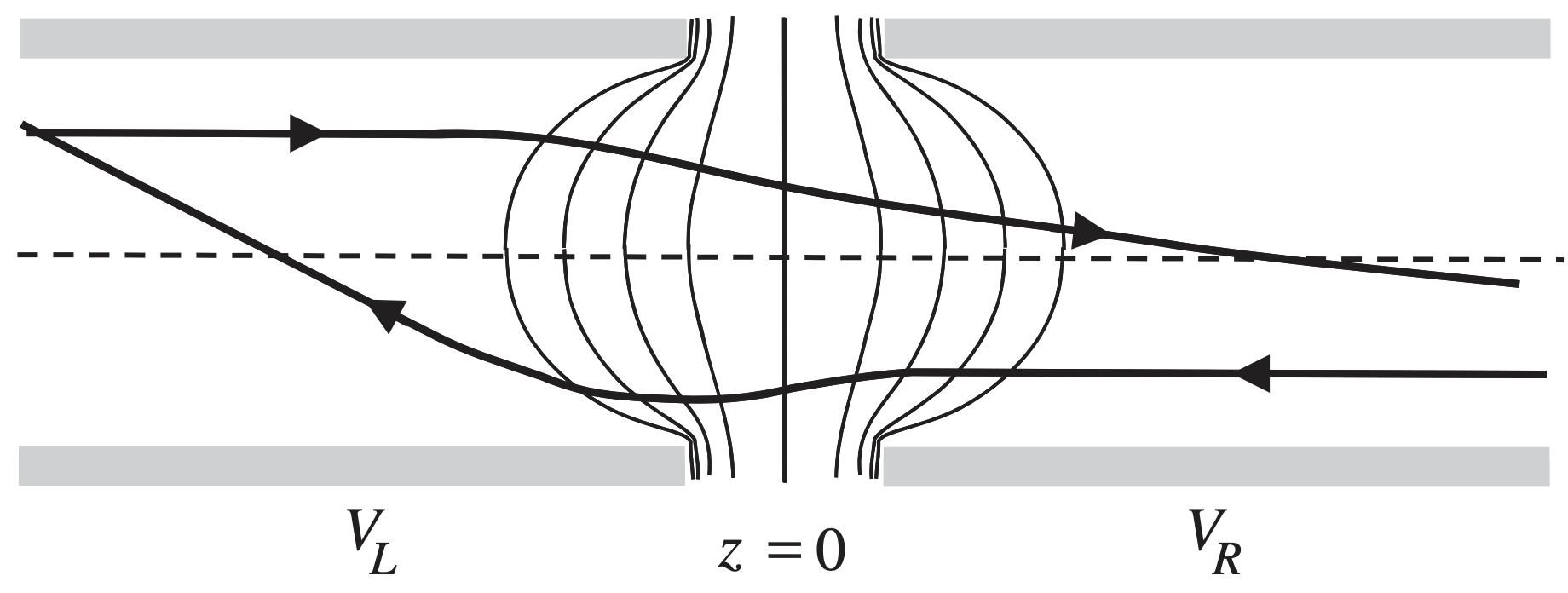
Example: Electrostatic Lens (Davisson & Calbick, 1931)

Phys. Rev. 38, 585 (1931). Two cylinders with gap at $z=0$, with constant potentials $V_L$ and $V_R$.

Regularity at origin and full angular range: $m=0$, only $I_0$.

$$\phi (\rho ,z)=\frac{1}{2\pi }{\int }_{-\infty }^{\infty }\mathrm{d}\kappa A(\kappa )I_0(|\kappa |\rho )e^{i\kappa z}+\text{const.}$$

with

$$A(\kappa )=\frac{1}{I_0(|\kappa |R)}{\int }_{-\infty }^{\infty }\mathrm{d}z\phi (R,z)e^{-i\kappa z}\text{.}$$

Regularizing the complex exponential, for a cylinder at potential $V_L$ for $z<0$ and $V_R$ for $z>0$:

$$\phi (\rho ,z)=\frac{V_R+V_L}{2}+\frac{V_R-V_L}{\pi }{\int }_0^{\infty }\frac{\mathrm{d}\kappa }{\kappa }\frac{I_0(\kappa \rho )}{I_0(\kappa R)}\sin (\kappa z)\text{.}$$

Why Converging Always Beats Diverging diverging (defocusing) effect is always weaker than the converging (focusing) one.

Near the symmetry axis of a cylindrical potential, the

Intuition: Near the axis, $I_0(\kappa \rho )\approx 1+(\kappa \rho {)}^2/4+\cdots$ so the radial field $E_{\rho }\propto \partial \phi /\partial \rho$ is proportional to $\rho$ (linear, lens-like). A charged particle traversing the lens spends more time in the converging region (where it slows down) than in the diverging region (where it speeds up). The time-weighted impulse from focusing always wins. This is the electrostatic analogue of the fact that a thin optical lens made of glass is always converging on net — because both surfaces bend light the same way for the dominant ray paths near axis.

The ${\int }_0^{\pm \infty }\mathrm{d}z{e}^{-i\kappa z}{e}^{\mp \alpha z}$ With $\alpha \to 0$ Trick

Several ways to motivate assigning ${\int }_0^{\infty }\mathrm{d}z{e}^{-i\kappa z}=\frac{1}{i\kappa }$:

1. Damped oscillation: ${\int }_0^{\infty }\mathrm{d}z{e}^{-i\kappa z}=\frac{1}{i\kappa }-{\lim }_{z\to \infty }\frac{e^{-i\kappa z}}{i\kappa }$; the oscillating tail carries no physical information.
2. Physical realism: No system is infinite; the answer should not depend on how we cut off at infinity.
3. Analytic continuation: When $\text{Im}(\kappa )<0$, the integral converges to $1/(i\kappa )$; take $\text{Im}(\kappa )\to 0$.
4. Distribution theory: ${\int }_0^{\infty }\mathrm{d}z{e}^{-i\kappa z}=\pi \delta (\kappa )+\frac{1}{i\kappa }$ in the distributional sense; the $\delta$-piece contributes the constant.

---

2D Polar Coordinates

For problems that are effectively two-dimensional, Laplace’s equation in polar coordinates $(\rho ,\varphi )$:

$$\frac{1}{\rho }\frac{\partial }{\partial \rho }\left(\rho \frac{\partial \phi }{\partial \rho }\right)+\frac{1}{{\rho }^2}\frac{{\partial }^2\phi }{\partial {\varphi }^2}=0$$

Separation gives ${\Phi }^{\prime \prime }=-{\alpha }^2\Phi$ and $R(\rho )={\rho }^{\pm \alpha }$ (for $\alpha \ne 0$), or $A+B\ln \rho$ and $C+D\varphi$ (for $\alpha =0$).

$\alpha \to i\alpha$ Example

For a region bounded by two arcs and two rays, ${\rho }^{\pm \alpha }$ cannot satisfy BCs. Instead, ${\rho }^{\pm i\gamma }=e^{\pm i\gamma \ln \rho }$, yielding oscillatory behavior in $\ln \rho$ paired with real exponentials (or $\sinh /\cosh$) in $\varphi$.

Example: Region ${\rho }_1<\rho <{\rho }_2$, ${\varphi }_1<\varphi <{\varphi }_2$:

$$\phi \propto \sin \left(\frac{m\pi \ln (\rho /{\rho }_2)}{\ln ({\rho }_1/{\rho }_2)}\right)\sinh \left(\frac{m\pi (\varphi -{\varphi }_1)}{\ln ({\rho }_1/{\rho }_2)}\right)$$

Wedge Singularity

$$\phi (\rho ,\varphi )=A+B\varphi +\sum _{\alpha }{C}_{\alpha }{\rho }^{\alpha }\sin (\alpha \varphi +{\delta }_{\alpha })\text{.}$$

For a grounded conducting wedge of opening angle $\beta$ ($A=B=0$, ${\delta }_{\alpha }=0$, $\alpha =m\pi /\beta$):

$$\phi (\rho ,\varphi )\sim {\rho }^{\pi /\beta }\sin \left(\frac{\pi \varphi }{\beta }\right)\text{near the apex}$$

The electric field $E\sim {\rho }^{(\pi /\beta )-1}$. For $\beta >\pi$ (reflex wedge / sharp edge), the field is singular as $\rho \to 0$.

The $\beta \to 2\pi$ limit (conducting half-plane / disk edge) gives $E\sim {\rho }^{-1/2}$ — the well-known square-root singularity of the surface charge density at a conductor’s edge.

---

Complex Potential

In 2D, ${\nabla }^2\phi =0$ means $\phi$ is the real (or imaginary) part of an analytic function $f(w)$ of $w=x+iy$.

Why Analyticity?

An analytic function has a derivative independent of direction in the complex plane. Choosing the $x$- and $y$-directions gives the Cauchy–Riemann equations:

$$\frac{\partial \phi }{\partial x}=\frac{\partial \psi }{\partial y},\frac{\partial \phi }{\partial y}=-\frac{\partial \psi }{\partial x}\text{.}$$

Both $\phi$ and $\psi$ individually satisfy Laplace’s equation. The CR equations also give $\nabla \phi \cdot \nabla \psi =0$, so curves of constant $\psi$ are field lines.

Write $f(w)=\phi +i\psi$ (the complex potential). The electric field is then:

$$\mathbf{E}=-\frac{df}{dw}\text{.}$$

Example — Uniform Field

$f(w)=-E_{0}w=-E_0(x+iy)$, so $\phi =-E_{0}x$ and field lines are $\psi =-E_{0}y=\text{const.}$

Conformal Mapping

Analytic functions generate conformal mappings $g(w)=u(x,y)+iv(x,y)$: a map from the $w=x+iy$ plane to the $g=u+iv$ plane that preserves angles and thus the property that equipotentials and field lines are orthogonal.

Strategy for awkward geometries: Find a conformal map that deforms the boundary into one where Laplace’s equation is trivial to solve. By Riemann’s mapping theorem, such a map exists (though the theorem is not constructive). In practice, extensive catalogues of known mappings cover many applications.

Conducting Strip in External Field

$$f(w)=\sqrt{w^2-a^2}=\phi +i\psi$$

• On the real axis with $|x|<a$: $\phi =0$ (grounded strip of width $2a$)
• For $|w|\gg a$: $f(w)\approx w$ (unit-strength uniform field at infinity)

This describes a uniform field perturbed by a 2D conducting plate.

Branch cut subtlety: $\sqrt{w^2-a^2}$ is not single-valued. Write $w+a=r_1{e}^{i{\theta }_1}$, $w-a=r_2{e}^{i{\theta }_2}$, then $f=\sqrt{r_1{r}_2}{e}^{i({\theta }_1+{\theta }_2)/2}$. The branch cut along $[-a,a]$ on the real axis ensures single-valuedness — and the resulting $\sigma \sim (a^2-x^2{)}^{-1/2}$ reproduces the square-root edge singularity.

Cylinder in Uniform Field (Prob. 7.25)

The Joukowski map $g=w+a^2/w$ maps the circle $|w|=a$ to the segment $|u|\le 2a$ on the real axis. The cylinder boundary becomes a flat plate.

On the plate ($v=0$): $\phi (u,0)=0$. Far away ($|g|\to \infty$, $g\approx w$): uniform field ${\mathbf{E}}_0\hat{v}$.

The trivial solution in the $g$-plane is $f(g)=i{E}_{0}g$, so $\phi =-E_{0}v$, $\psi =E_{0}u$.

Mapping back: $g=w+a^2/w$ with $w=x+iy$:

$$\phi (x,y)=-E_{0}y\left(1-\frac{a^2}{x^2+y^2}\right)$$

which is the well-known result for a cylinder in a uniform field, obtained without solving any boundary-value problem directly.

Can We Get This Without Conformal Mapping?

Yes — by direct separation in cylindrical coordinates. The $\cos \varphi$ angular dependence is forced by the uniform-field BC at infinity, giving $\phi =(-E_{0}r+B/r)\cos \varphi$. Imposing $\phi (a,\varphi )=0$ gives $B=E_0{a}^2$, recovering the same result.

Fringing Field of a Capacitor

The conformal mapping approach also gives the fringing field of a parallel-plate capacitor — one of the examples worked out in Maxwell’s Treatise. The mapping deforms the semi-infinite plate geometry into a tractable domain.

The complex-potential method extends naturally to systems with explicit line sources (line charges, wire arrays, line dipoles): see Chapter 8 for the wire chamber, alternating-line arrays, and conformal-mapping image constructions.

---

Variational Method

Recalling Thomson’s Theorem

Thomson's Theorem

Among all charge distributions $\rho (\mathbf{r})$ with total charge $Q$ in a volume $V$, the electrostatic energy is minimized when the potential is constant throughout $V$ (i.e., the charge resides on the surface, as on a conductor).

Variational Principle for Laplace’s Equation

Energy Minimization Principle

Among all potential functions $\phi (\mathbf{r})$ that take prescribed values on a set of bounding surfaces, the electrostatic energy

$$U_E[\phi ]=\frac{{ϵ}_0}{2}\int {\mathrm{d}}^{3}r|\mathbf{E}{|}^2$$

is minimized by the $\phi$ satisfying Laplace’s equation.

Proof Sketch

Let $\phi$ be the true solution and $\psi =\phi +\delta \phi$ a variation. Then:

$$U_E[\psi ]-U_E[\phi ]={ϵ}_0\int {\mathrm{d}}^{3}r\nabla \phi \cdot \nabla (\delta \phi )+\frac{{ϵ}_0}{2}\int {\mathrm{d}}^{3}r|\nabla (\delta \phi ){|}^2\text{.}$$

The first term: integrate by parts. The volume integral gives $-\int {\mathrm{d}}^{3}r\delta \phi {\nabla }^2\phi =0$ (Laplace). The surface integral gives $\oint \mathrm{d}S\delta \phi {\partial }_n\phi =0$ because:

• Dirichlet: $\delta \phi =0$ on boundaries;
• Neumann: ${\partial }_n\phi$ is prescribed, so it doesn’t vary.

The remaining term $\frac{{ϵ}_0}{2}\int {\mathrm{d}}^{3}r|\nabla (\delta \phi ){|}^2>0$ is manifestly positive.

(Prescribed constant values on boundaries not even necessary — works for general Dirichlet and Neumann.)

Practical Procedure

Construct a trial solution $\psi (\mathbf{r};p_1,p_2,\dots )$ satisfying all BCs, depending on adjustable parameters. Minimize $U_E[\psi ]$ with respect to $\{p_i\}$.

Why This Is Practical

The resulting energy differs from the exact energy by an amount quadratic in the difference $\psi -\phi$. This is significant because applications often demand accuracy in energy or force rather than in the potential itself. Accuracy can be improved arbitrarily by adding more variational parameters to $\psi$.

On Minimizing a Partial Energy (Zangwill Example 7.5)

In the rectangular slot example, Zangwill minimizes only the energy inside the slot, not the total energy of the entire system. This is valid because: as we vary the trial parameter $p$, the field outside the slot is entirely determined by the boundary values (which are fixed). The total energy is $U_{\text{inside}}(p)+U_{\text{outside}}$. Since $U_{\text{outside}}$ is independent of $p$, minimizing $U_{\text{inside}}(p)$ is equivalent to minimizing $U_{\text{total}}(p)$.

---

Problems

Foundations

7.2 — Green’s Formula

At a point $P$ on an equipotential surface with principal radii of curvature $R_1$ and $R_2$, show that the electric field satisfies $\partial E_n/\partial n=-2\kappa E_n$, where $\kappa =\frac{1}{2}(R_1^{-1}+R_2^{-1})$ is the mean curvature and $\hat{n}$ is the outward normal.

Solution Sketch

$\hat{n}$ is normal to an equipotential at point $P$ with principal radii of curvature $R_1,R_2$.

Method 1 (Local coordinates $x$ and $y$): Equipotential surface $n=\frac{x^2}{2R_1}+\frac{y^2}{2R_2}$ near $P$ (from $x^2+(n-R{)}^2=R^2$). Laplace’s equation with $z=n$ and chain rule gives the mean curvature relation.

Method 2 (Differential geometry): Mean curvature $\kappa =\frac{1}{2}\left(\frac{{\partial }^{2}z}{\partial x^2}+\frac{{\partial }^{2}z}{\partial y^2}\right){|}_P$, and $2\kappa =\nabla \cdot \hat{n}$. Combined with ${\nabla }^2\phi =0$ directly yields the identity:

$$\frac{\partial E_n}{\partial n}=-2\kappa E_n\text{.}$$

Physical Insight

• $\kappa >0$: field lines diverge, $E_n$ decreases along them
• Reduces the problem to a 1D ODE along a field line if we know the equipotential geometry
• Near sharp conductors: high curvature → rapid spatial variation of $E$

7.3 — Poisson’s Formula for a Sphere

Derive an expression for the potential at any point inside a sphere of radius $R$ purely in terms of the potential on the sphere’s surface — without knowing the charge distribution that produces it.

Solution Sketch

Interesting because we only need $\phi$ on the sphere surface.

Trick: Use the identity

$$r{\partial }_r\frac{1}{|\mathbf{r}-{\mathbf{r}}_S^{\prime }|}-R{\partial }_R\frac{1}{|\mathbf{r}-{\mathbf{r}}_S^{\prime }|}=\frac{R^2-r^2}{|\mathbf{r}-{\mathbf{r}}_S^{\prime }{|}^3}\text{.}$$

On the other side (expanding in Legendre polynomials), this produces $(2\ell +1)r^{\ell }/R^{\ell +1}{P}_{\ell }(\cos \gamma )$. After integration over the surface and orthogonality selecting out the full potential:

$$\phi (\mathbf{r})=\frac{R(R^2-r^2)}{4\pi }\oint \frac{\phi ({\mathbf{r}}_S^{\prime })}{|\mathbf{r}-{\mathbf{r}}_S^{\prime }{|}^3}d{S}^{\prime }\text{.}$$

7.4 / 7.5 — Symmetry Elimination

Given a charge or boundary configuration with discrete symmetries (reflection, rotation), determine which spherical harmonic terms $Y_{\ell }^m$ are forced to vanish before solving Laplace’s equation.

Solution Sketch

Many terms can be eliminated by symmetry considerations alone before imposing Laplace’s equation. Identify the point group of the geometry → kill all harmonics that don’t transform as the trivial representation under the surviving symmetries → then impose ${\nabla }^2\phi =0$ on what remains.

Cartesian

7.6 — The Microchannel Plate

Two sets of interleaved conducting strips at $x=0$ and $x=d$, infinite in extent, with neighboring strips separated by $b$ in the $y$-direction and differing in potential by a fixed amount (taken as 2). Find $\phi (x,y)$ in the gap.

Solution Sketch

Periodicity in $y$: $\phi (x,y+b)=\phi (x,y)+2$ (potential increments by a fixed amount per period).

Enforce with $\phi (x,y)=\frac{2y}{b}+f(x,y)$ where $f$ is $b$-periodic. The linear term captures the average gradient; $f$ provides oscillatory corrections (effectively a sawtooth decomposition).

In $x$: $\sinh$ and $\cosh$ terms. Since the period is $b$: ${\alpha }_m=2\pi m/b$.

Integrate over a single strip on, e.g., the lower plate ($\phi =0$ is easiest). Use orthogonality to isolate $A_m$ and $B_m$.

Strategy: Keep track of which parameters carry indices. It’s easiest to write $\sin$, $\cos$, $\sinh$, $\cosh$; argue from symmetry for just $\sin ({\alpha }_{m}y)$; then find $\sinh /\cosh$ coefficients from the $x$-boundary conditions.

7.7 — A Potential Patch by Separation of Variables

A grounded conducting plane at $z=d$ and a conducting plane at $z=0$ which is grounded everywhere except on a square patch $|x|<a$, $|y|<a$, held at potential $V$. Find $\phi (x,y,z)$ in the region $0<z<d$.

Solution Sketch

The inhomogeneous BC direction ($z$) gets the hyperbolic function, shifted to vanish at $z=d$. Symmetry gives $\cos (k_{x}x)\cos (k_{y}y)$.

$$\phi =\frac{V}{{\pi }^2}\int \mathrm{d}{k}_x\frac{\sin (k_{x}a)\cos (k_{x}x)}{k_x}\int \mathrm{d}{k}_y\frac{\sin (k_{y}a)\cos (k_{y}y)}{k_y}\frac{\sinh (\sqrt{k_x^2+k_y^2}(d-z))}{\sinh \left(\sqrt{k_x^2+k_y^2}d\right)}$$

The coefficients don’t factorize — the source geometry couples $k_x$ and $k_y$ through the $z$-dependence.

7.8 — A Conducting Slot

A semi-infinite rectangular slot of width $a$ extends from $z=0$ to $z\to \infty$, with the two side walls ($x=0$ and $x=a$) grounded. The base at $z=0$ is held at constant potential ${\phi }_0$. Find $\phi (x,z)$.

Solution Sketch

Linear terms vanish. In $x$: oscillatory, vanishing at $0$ and $a$ gives $\sin (m\pi x/a)$. In $z$: only $e^{-\alpha z}$ for regularity.

$$\phi (x,z)=\frac{2{\phi }_0}{\pi }\sum _{m\text{odd}}\frac{1}{m}\sin \left(\frac{m\pi x}{a}\right)e^{-m\pi z/a}\text{.}$$

Dominant term ($m=1$): influence of the source charge reaches distances of order $a$. Transverse variations also vary on scale $\sim a$, which makes sense: the slot width is the only characteristic length of the problem.

7.9 — A Two-Dimensional Potential Problem in Cartesian Coordinates

Two semi-infinite conducting planes at $z=\pm d$ extend in opposite $x$-directions, held at potentials $+V$ and $-V$ respectively. Find $\phi$.

Solution Sketch

$\phi (x,y,z)=\phi (x,z)$ (no $y$-dependence).

• $\phi (-x,z)=-\phi (x,z)$ → $\sin (kx)$ only
• $\phi (x,-z)=\phi (x,z)$ → no linear term in $z$; use $\cosh (kz)$

Since $x$ is infinite, we insist on a Fourier representation: integrate over sine components only ($\sin$ is selected by odd symmetry), which gives an integral over $k\in [0,\infty )$. The cosine in $z$ is selected by even symmetry.

Spherical

7.10 — An Electrostatic Analog of the Helmholtz Coil

Two nonconducting strips are painted on a sphere of radius $R$, symmetric about the equator, each of angular half-width $w$ centered at colatitudes ${\theta }_0$ and $\pi -{\theta }_0$, held at potentials $+V$ and $-V$. Find the angle ${\theta }_0$ that makes the interior electric field maximally uniform.

Solution Sketch

Nonconducting strips → single solution valid for the whole range. No azimuthal dependence ($m=0$).

$$\phi (r,\theta )=\sum _{\ell }{A}_{\ell }{r}^{\ell }{P}_{\ell }(\cos \theta )$$ $$A_{\ell }=\frac{V(2\ell +1)}{w{R}^{\ell }}[1-(-1{)}^{\ell }]{\int }_0^{{\theta }_0}\mathrm{d}\theta \sin \theta P_{\ell }(\cos \theta )$$

The $\ell =1$ term gives a uniform $\hat{z}$ field.

To eliminate the leading nonuniform correction ($\ell =3$): set $5{\cos }^4{\theta }_0-6{\cos }^3{\theta }_0-1=0$

$$\Rightarrow {\cos }^2{\theta }_0=\frac{1}{5}\Rightarrow {\theta }_0\approx 63.4°$$

Source: C.E. Baum, IEEE Trans. Electromagnetic Compatibility 30, 9 (1988).

7.11 — Make a field inside a Sphere

Given the potential inside a sphere (expressed as a sum of $r^{\ell }{Y}_{\ell }^m$ terms), find the potential outside by matching at $r=R$.

Solution Sketch

Once we have the field inside, the outside is immediate: match potentials and swap $r^{\ell }\to r^{-(\ell +1)}$.

7.12 — The Capacitance of an Off-Center Capacitor

Two conducting spheres of radii $R_1<R_2$, nominally concentric, with centers displaced by a small distance $s$. The inner sphere is at potential $V$ and the outer is grounded. Find the capacitance $C(s)$ to leading nontrivial order in $s$.

Solution Sketch

$R_2^2=s^2+r_2^2-2s{r}_2\cos \theta ⟹r_2\approx R_2+s\cos \theta$ for small displacement $s$.

Ansatz: $\phi \sim a+b/r+s(cr+d/r^2)+\mathcal{O}(s^2)$. Alternatively, approximate $r^{\ell }$ and $r^{-(\ell +1)}$ on the $r_2$ surface; for $\ell \ne 0$, coefficients $\propto s$ (from recurrence relations connecting different orders).

Key observation: Due to $\cos \theta$ angular dependence, the first-order correction to $Q$ drops out (as expected: $C$ doesn’t change to first order).

To find $C$ via $Q/\Delta V$, we’d need second-order corrections ($A_2,B_2$).

Cleverer approach — bootstrapping to second order:

$$F_s=\frac{1}{2}(\Delta V{)}^2\frac{\mathrm{d}C}{\mathrm{d}s}\text{.}$$

This gives us the derivative of $C$, and hence the second-order correction to $C$, using only first-order results!

Even better: since $Q$ is invariant, $\frac{\mathrm{d}}{\mathrm{d}s}\frac{Q^2}{2C}\propto \frac{\mathrm{d}C}{\mathrm{d}s}\propto F_z$. Integrating from $C_0$ to $C(s)$:

$$C=C_0\left(1-\frac{C_0}{4\pi {ϵ}_0}\frac{s^2}{R_2^3-R_1^3}\right)\text{.}$$

7.13 — The Plane–Cone Capacitor

A conducting cone of half-angle $\pi /4$ shares its apex with an infinite conducting plane. The cone is at potential $V$; the plane is grounded. Find $\phi (\theta )$ in the gap (which has azimuthal symmetry and scaling invariance).

Solution Sketch

Between the plates: no $\rho$-dependence (scaling invariance), no $\varphi$-dependence (azimuthal symmetry). Just the $\theta$-part of Laplace, which integrates directly:

$$\phi (\theta )=V\frac{\ln \tan (\theta /2)}{\ln \tan (\pi /8)}\text{.}$$

7.14 — A Conducting Sphere at a Dielectric Boundary

Conducting sphere of radius $R$ with charge $Q$ centered at origin + two linear dielectric regions (boundary $z=0$) with constants ${\kappa }_1$ ($z>0$) and ${\kappa }_2$ ($z<0$). Find $\phi (r>R)$.

Solution Sketch

$\mathbf{P}\sim \hat{r}/r^2$ gives a $\delta$-function polarization charge, but this is outside the region. No boundary charges at the dielectric discontinuity because fields are radial everywhere — polarization charge is compensated at infinity.

$$\phi (r>R)=\frac{Q}{r}\frac{1}{2\pi {ϵ}_0({\kappa }_1+{\kappa }_2)}$$

Check: ${\kappa }_1={\kappa }_2=1⟹{\kappa }_1+{\kappa }_2=2$, recovering the expected vacuum result.

7.15 — Force on an Inserted Conductor

Inside volume $r<a$: ${\varphi }_{\text{ext}}(r,\theta )={\sum }_{n=1}^{\infty }{\alpha }_n{\left(\frac{r}{R}\right)}^n{P}_n(\cos \theta )$. Insert solid conducting sphere of radius $R<a$ at the origin and show that the force exerted on it when it’s grounded is:

$$F_z=4\pi {\epsilon }_0\sum _{n=1}^{\infty }(n+1){\alpha }_n{\alpha }_{n+1}\text{.}$$

Legendre polynomials recurrence relation:

$$(n+1)P_{n+1}(x)+n{P}_{n-1}(x)=(2n+1)x{P}_n(x)\text{.}$$

Solution Sketch

From the external solution, we know the internal as well. Integrate the force density over the sphere surface, or use the stress tensor: the $\theta$-components drop because $(r/R{)}^n-(R/r{)}^{n+1}$ vanishes at $r=R$, leaving only:

$$T_{rr}=\frac{{ϵ}_0}{2}(E_r^2-\frac{1}{2}{E}_r^2)=\frac{{ϵ}_0}{2}{E}_r^2\cdot \frac{1}{2}\text{.}$$

(Only the radial component of the Maxwell stress survives on the surface.)

Cylindrical

7.16 — A Segmented Cylinder

Infinite cylinder with $2\alpha$ angular range held at unit potential, the rest at zero potential.

Solution Sketch

$\phi (\rho ,-\varphi )=\phi (\rho ,\varphi )$ → only $\cos (m\varphi )$ terms. Regularity at origin: $(\rho /R{)}^m$.

$$\phi (\rho ,\varphi )=\frac{\alpha }{\pi }+\frac{2}{\pi }\sum _{m=1}^{\infty }\frac{1}{m}{\left(\frac{\rho }{R}\right)}^m\sin (m\alpha )\cos (m\varphi )\text{.}$$

7.17 — An Incomplete Cylinder

A conducting cylindrical shell of radius $R$ subtends an angle $2\pi /p$ (i.e., it is a fraction $1/p$ of a full cylinder) and carries total charge $Q$ per unit length. Find how the charge distributes between the inner and outer surfaces.

Solution Sketch

Even though the cylinder is incomplete, Laplace’s equation holds for the whole $0\le \varphi \le 2\pi$ range → no linear $\varphi$ term.

Interior: ${\phi }_{\text{in}}=A_0+{\sum }_n{\left(\frac{\rho }{R}\right)}^n{G}_n(\varphi )\text{.}$

Exterior: ${\phi }_{\text{out}}=A_0-\frac{\lambda }{2\pi {ϵ}_0}\ln \left(\frac{\rho }{R}\right)+{\sum }_n{A}_n{\left(\frac{R}{\rho }\right)}^n{G}_n(\varphi )\text{.}$

where $G_n$ is a linear combination of $e^{\pm in\varphi }$. The charge on each side corresponds to derivatives of potential in the two limits.

Result:

$$\frac{Q_{\text{tot}}-Q_{\text{in}}}{Q_{\text{tot}}}=\frac{1}{2}\left(1-\frac{1}{p}\right)\text{.}$$

Check: For $p=1$ (complete cylinder), this gives zero — all charge is on the outer shell, as expected.

7.18 — The Two-Cylinder Electron Lens

A conducting cylinder of radius $R$ is held at potential $V_L$ for $z<0$ and $V_R$ for $z>0$ (with a thin insulating gap at $z=0$). Find $\phi (\rho ,z)$ inside.

Solution Sketch

Regularity at origin + azimuthal independence: $J_0(k\rho )$ with $e^{-k|z|}$. BCs: $V_L$ for $z<0$, $V_R$ for $z>0$. Continuity at $z=0$ gives $V_L-V_R=2{\sum }_n{B}_n{J}_0(k_n\rho )$.

$$\phi (\rho ,z)=\frac{V_R+V_L}{2}+\mathrm{sgn}(z)\left[\frac{V_L-V_R}{2}-(V_L-V_R)\sum _n\frac{J_0(k_n\rho )}{k_{n}R{J}_1(k_{n}R)}{e}^{-k_n|z|}\right]\text{.}$$

Bessel identities used:

$$\lambda {\int }_0^1\mathrm{d}ss{J}_0(\lambda s)=J_1(\lambda )\text{;}$$ $$2{\int }_0^1\mathrm{d}ss{J}_0(x_{n}s)J_0(x_{m}s)=J_1^2(x_n){\delta }_{mn}\text{.}$$

7.19 — A Periodic Array of Charged Rings

A periodic array of thin charged rings (total charge $Q$ each, spacing $b$) sits on the axis of a grounded conducting cylinder of radius $R$. Find $\phi (\rho ,z)$ and verify that the limiting form far from any ring reproduces the expected line-charge behavior $\lambda =Q/b$.

Solution Sketch

Azimuthal symmetry → only $I_0$ and $K_0$ terms. Place $K_0(\cdot R)$ and $I_0(\cdot R)$ respectively in each region to facilitate BC matching.

Matching uses the Wronskian identity:

$$I_{\alpha }^{\prime }(y)K_{\alpha }(y)-I_{\alpha }(y)K_{\alpha }^{\prime }(y)=\frac{1}{y}$$

Limiting case gives a logarithmic term of an apparent line charge $\lambda =Q/b$.

This is a useful diagnostic: if the edge case reveals a $\ln \rho$ term that you didn’t include from the start, it signals you missed the $k=0,\alpha =0$ sector of the separation. Always check limiting cases against expected multipole behavior.

7.20 — Axially Symmetryc Potentials

Prove that for any azimuthally symmetric potential, the off-axis values can be reconstructed from the on-axis potential alone via:

$$V(\rho ,z)=\frac{1}{\pi }{\int }_0^{\pi }\mathrm{d}\xi V(z+i\rho \cos \xi )\text{.}$$

Solution Sketch

$$V(\rho ,z)=\frac{1}{\pi }{\int }_0^{\pi }\mathrm{d}\xi V(z+i\rho \cos \xi )\text{.}$$

Interpretation: The off-axis potential is a harmonic average of the “analytically continued” on-axis potential over a path that reaches into the complex plane by an amount proportional to $\rho$.

Connection to Legendre expansion: On axis, $\phi (0,0,z)={\sum }_n{a}_n{z}^n$. Each $a_n{z}^n$ generates the Legendre polynomials that appear in the full azimuthally symmetric expansion. The integral acts as a harmonic continuation operator — non-harmonic parts cancel upon integration.

This is essentially the converse of the generating-function trick: instead of going from full solution → axis, we go from axis → full solution.

2D and Special

7.21 — Two Disks

Two coaxial conducting disks of radius $a$, separated by $2L$, held at potentials $\pm V$. Examine the solution proposed in a paper and show why it’s lacking.

Solution Sketch

Laplace’s equation in three regions (inner region has both exponential terms in $z$). Matching at both disk surfaces gives:

$$\phi \propto e^{-k|z-L|}-e^{-k|z+L|}$$

Subtlety: The discontinuity $2{\int }_0^{\infty }\mathrm{d}kkA(k)J_0(k\rho )$ does not vanish for $\rho \ge a$ (which is vacuum). The potential itself is continuous but its normal derivative need not be — the integral equation enforces the mixed boundary condition (Dirichlet on the disk, continuity off the disk).

Source: B.D. Hughes, J. Phys. A 17, 1385 (1985).

7.22 — A Dielectric Wedge in Polar Coordinates

Two wedge shaped dielectrics held at different potentials share a common edge ($\varphi =0$). Find $\phi$.

Solution Sketch

Scaling invariance → no $\rho$-dependence. The solution reduces to $\phi =A+B\varphi$ in both angular regions. Match at the boundaries.

7.23 — Contact Potential

Two coplanar conducting half-planes at $\varphi =0$ and $\varphi =\pi$ (separated by $y=0$) are held at potentials $0$ and $V$ respectively. Find $\phi$ and $\mathbf{E}$.

Solution Sketch

Scaling invariance → no $\rho$-dependence. Just $A+B\varphi$ again.

$$\mathbf{E}=-\frac{V}{\pi }\frac{\hat{\varphi }}{\rho }$$

Physical insight: The $1/\rho$ field is the same as that of a line charge — but here it arises purely from geometry. The field is azimuthal, not radial, and the $1/\rho$ dependence is dictated by scaling invariance: in the absence of any length scale, the field must fall off as $1/\rho$ on dimensional grounds.

---

Cross-Chapter Connections

• Green functions (Ch. 8): Systematic way to handle arbitrary BCs once the geometry’s Green function is known
• Method of images (Ch. 8): Shortcut for conductors with simple geometries — leverages uniqueness
• Multipole expansion (Ch. 4): The exterior spherical solution is the multipole expansion
• Steady currents (Ch. 9): Same Laplace equation, Neumann BCs arise naturally
• Magnetostatics (Ch. 11): Magnetic scalar potential satisfies Laplace outside currents
• Meissner effect (Ch. 13): Neumann BC for magnetic potential at superconductor surfaces

TODO: Fix Cross-Chapter Connections.

TODO: Overview and/or common pitfalls.

TODO: Review problems.

TODO: Exact problem statements.